Chapter 6 TD Learning
Temporal-Difference Learning is defined here as central to reinforcement learning.
Tabular TD(0) Prediction
Use temporal difference to estimate the state value function of a given policy.
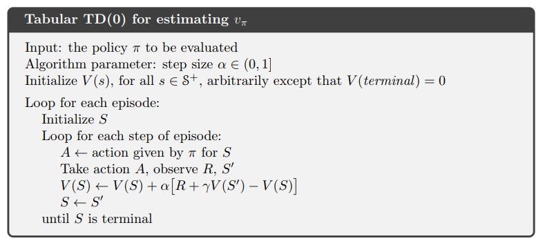
In IntroRL, the main loop of the TD(0) Prediction is shown below.
while (num_episodes<=max_num_episodes-1) and keep_looping:

    keep_looping = False
    abserr = 0.0 # calculated below as part of termination criteria

    # policy evaluation
    for start_hash in start_stateL:
        num_episodes += 1
        if num_episodes > max_num_episodes:
            break

        s_hash = start_hash
        a_desc = policy.get_single_action( s_hash )
        for _ in range( max_episode_steps ):

            sn_hash, reward = Env.get_action_snext_reward( s_hash, a_desc )

            state_value_coll.td0_update( s_hash=s_hash, alpha=alpha_obj(),
                                                     gamma=gamma, sn_hash=sn_hash,
                                                     reward=reward)

            if (sn_hash in Env.terminal_set) or (sn_hash is None):
                break

            # get ready for next step
            s_hash = sn_hash

            a_desc = policy.get_single_action( s_hash )
            if a_desc is None:
                print('a_desc is None for policy.get_single_action( "%s" ) ='%\
                      str(s_hash), a_desc)

    abserr = state_value_coll.get_biggest_action_state_err()
    if abserr > max_abserr:
        keep_looping = True

    if num_episodes < min_num_episodes:
        keep_looping = True # must loop for min_num_episodes at least
Example 6.2 Random Walk
Example 6.2 in Sutton & Barto on page 125 uses the random walk Markov Reward Process (MRP) below.
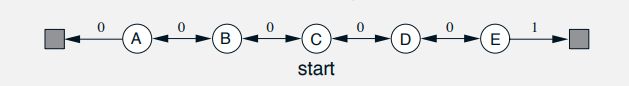
The solution from Sutton & Barto and from IntroRL are shown below.
They both show that TD(0) converges more quickly than MC for this problem.


Figure 6.2 Batch Training
Figure 6.2 on page 127 of Sutton & Barto shows that batch TD is consistently better than batch MC for the random walk shown above in example 6.2.
The figure on the left below is directly from Sutton & Barto
The figure on the right below is generated by IntroRL and overlays the results of IntroRL, Sutton & Barto and Shangtong Zhang


Sarsa On-Policy TD Control
Baseline for epsilon greedy version of Sarsa.
The pseudo code of SARSA prediction of Q(s,a) is given on page 130 of Sutton & Barto and is shown below.
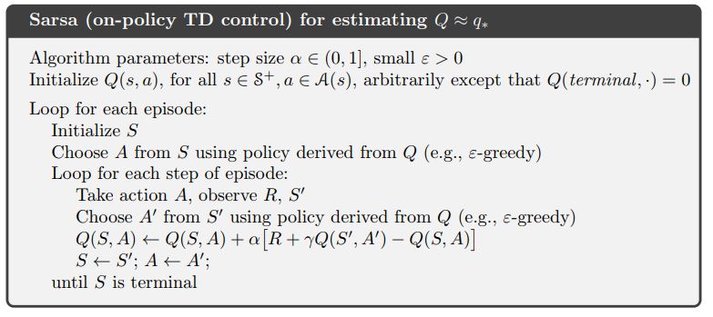
The main loop of the IntroRL Epsilon Greedy Sarsa control function is shown below
while (episode_loop_counter<=max_num_episodes-1) and keep_looping :

    keep_looping = False
    abserr = 0.0 # calculated below as part of termination criteria
    Nterminal_episodes = set() # tracks if start_hash got to terminal_set or max_num_episodes

    for start_hash in loop_stateL:
        episode_loop_counter += 1
        if episode_loop_counter > max_num_episodes:
            break

        if learn_tracker is not None:
            learn_tracker.add_new_episode()

        s_hash = start_hash
        a_desc = action_value_coll.get_best_eps_greedy_action( s_hash, epsgreedy_obj=eg )

        for n_episode_steps in range( max_episode_steps ):

            # Begin an episode
            if a_desc is None:
                Nterminal_episodes.add( start_hash )
                print('break for a_desc==None')
                break
            else:
                sn_hash, reward = environment.get_action_snext_reward( s_hash, a_desc )
                if learn_tracker is not None:
                    learn_tracker.add_sarsn_to_current_episode( s_hash, a_desc,
                                                                reward, sn_hash)

                if sn_hash is None:
                    Nterminal_episodes.add( start_hash )
                    print('break for sn_hash==None')
                    break
                else:
                    an_desc = action_value_coll.get_best_eps_greedy_action( sn_hash,
                                                                            epsgreedy_obj=eg )

                    action_value_coll.sarsa_update( s_hash=s_hash, a_desc=a_desc,
                                                    alpha=alpha_obj(), gamma=gamma,
                                                    sn_hash=sn_hash, an_desc=an_desc,
                                                    reward=reward)

                    if sn_hash in environment.terminal_set:
                        Nterminal_episodes.add( start_hash )
                        if (n_episode_steps==0) and (num_s_hash>2):
                            print('1st step break for sn_hash in terminal_set', sn_hash,
                                  ' s_hash=%s'%str(s_hash), ' a_desc=%s'%str(a_desc))
                        break
                    s_hash = sn_hash
                    a_desc = an_desc

    # increment episode counter on EpsilonGreedy and Alpha objects
    eg.inc_N_episodes()
    alpha_obj.inc_N_episodes()

    abserr = action_value_coll.get_biggest_action_state_err()
    if abserr > max_abserr:
        keep_looping = True

    if episode_loop_counter < min_num_episodes:
        keep_looping = True # must loop for min_num_episodes at least
Example 6.5 Windy Gridworld
Example 6.5 applies epsilon greedy Sarsa to the Windy Gridworld
The case is run with gamma=1.0, epsilon=0.1 and alpha=0.5 Example 6.5 Windy Gridworld, Full Souce Code
Shown below on the left is the answer published in Sutton & Barto
On the right is a plot comparing the results if IntroRL, Sutton & Barto and Denny Britz


The policy from the IntroRL run results in the episode shown below, however, the resulting policy was not consistent, often getting caught in infinite loops:
 _________________ Windy Gridworld Sutton Ex6.5 Episode Summary ________________
      *       *       *       *       *       *  [7->R]  [8->R]  [9->R] [10->D]  ||
      *       *       *       *       *  [6->R]       *       *       * [11->D]  ||
      *       *       *       *  [5->R]       *       *       *       * [12->D]  ||
 [1->R]  [2->R]  [3->R]  [4->R]       *       *       *       *       * [13->D]  ||
      *       *       *       *       *       *       *       * [15->L] [14->L]  ||
      *       *       *       *       *       *       *       *       *       *  ||
      *       *       *       *       *       *       *       *       *       *  ||
___0_______0_______0_______1_______1_______1_______2_______2_______1_______0___
 ______________________________ Upward Wind Speed ______________________________
Example 6.6 Cliff Walking
Example 6.6 compares epsilon-greedy Q-learning to epsilon-greedy Sarsa for a Cliff Walking Gridworld. The Q-learning pseudo code is given on page 131 of Sutton & Barto
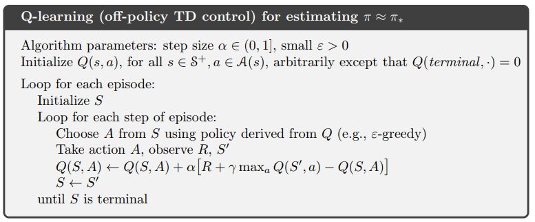
The Example 6.6 Cliff Walking, Full Souce Code of the IntroRL Q-learning function is much like the Sarsa On-Policy, Full Souce Code except for the update of the Q(s,a) value.
# Q-learning Q(s,a) update
action_value_coll.qlearning_update( s_hash=s_hash, a_desc=a_desc, sn_hash=sn_hash,
                                    alpha=alpha_obj(), gamma=gamma,
                                    reward=reward)

# Sarsa Q(s,a) update
action_value_coll.sarsa_update( s_hash=s_hash, a_desc=a_desc,
                                alpha=alpha_obj(), gamma=gamma,
                                sn_hash=sn_hash, an_desc=an_desc,
                                reward=reward)
The point of Example 6.6 is to show that Sarsa takes the epsilon-greedy action selection into account and travels the safer route along the top of the grid.
Q-learning takes the more efficient route along the edge of the cliff, ignoring the exploration dangers of epsilon-greedy.
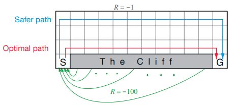


The above-right image overlays the results of Sutton & Barto and IntroRL.
Figure 6.3 Expected Sarsa
Figure 6.3 on page 133 of Sutton & Barto illustrates the benefit of Expected Sarsa over both Sarsa and Q-learning.
The description of figure 6.3 applies to the chart on the left, below.
The chart on the right is run by IntroRL with fewer runs than the Sutton & Barto chart.


The plot above is created by first running a script to make a data file, Make Figure 6.3 Expected Sarsa Data File Code
And then running a script to create the plot, Figure 6.3 Expected Sarsa, Plotting Souce Code
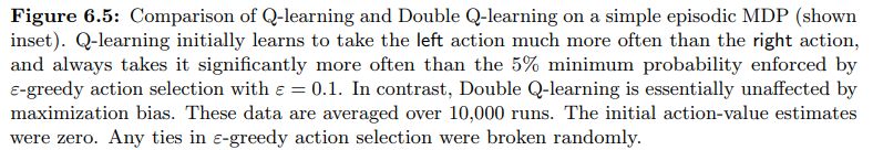
Figure 6.5 Double Qlearning
Double Q-learning is outlined in the pseudo code below.
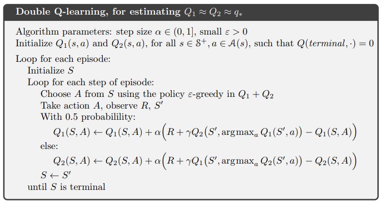
Figure 6.5 demonstrates how Double Qlearning is virtually unaffected by maximization bias.


The IntroRL chart, above right, was run with 10 choices from (B) in the MDP Figure 6.5 Double Qlearning, Full Souce Code
The IntroRL values are overlaid on the Sutton & Barto values.