Chapter 4 DP
Dynamic Programming, DP, is a collection of algorithms that can be used to solve MDPs.
DP provides approaches to compute value functions, V(s). The four major approaches are:
(1) Policy Evaluation  - given a policy calc V(s)
(2) Policy Improvement - given V(s) calc policy
(3) Policy Iteration   - calc policy and V(s) by alternating (1) and (2)
(4) Value Iteration    - calc policy and V(s) with more efficient (3)
IntroRL provides functions for all four of the above algorithms.
Policy Evaluation
The approach to policy evaluation is defined in Sutton & Barto pages 74 and 75 as follows.
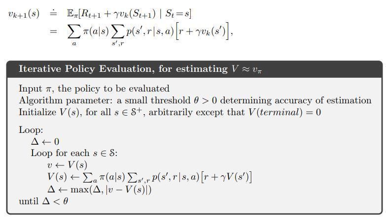
The main loop of the policy evaluation code in IntroRL is shown below.
while (loop_counter<max_iter) and (not all_done):
    loop_counter += 1
    all_done = True
    delta = 0.0 # used to calc largest change in state_value

    # policy evaluation
    for s_hash in policy.iter_all_policy_states():

        calcd_v = 0.0
        for a_desc, a_prob in policy.iter_policy_ap_for_state( s_hash, incl_zero_prob=False):

            for sn_hash, t_prob, reward in \
                Env.iter_next_state_prob_reward(s_hash, a_desc, incl_zero_prob=False):

                calcd_v += t_prob * a_prob * ( reward + gamma * state_value(sn_hash) )

        delta = max( delta, abs(calcd_v - state_value(s_hash)) )
        if delta > error_limit:
            all_done = False
            max_delta = max(max_delta, delta) # returned to caller

        state_value[s_hash] = calcd_v
Policy Improvement
The approach to policy evaluation is defined in Sutton & Barto pages 76 to 80 as follows.
It finds the greedy policy consistent with the current value function, V(s), discount factor, gamma and the MDP behavior.
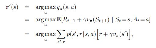
The main loop of the policy improvement code in IntroRL is shown below.
while (loop_counter<max_iter) and (not is_stable):
    loop_counter += 1
    is_stable = True

    # policy improvement
    for s_hash in policy.iter_all_policy_states():
        old_action = policy.get_single_action( s_hash )

        VsD = {} # will hold: index=a_desc, value=V(s) for all transitions of a_desc from s_hash
        for a_desc, a_prob in policy.iter_policy_ap_for_state( s_hash, incl_zero_prob=True):
            VsD[a_desc] = 0.0
            for sn_hash, t_prob, reward in \
                Env.iter_next_state_prob_reward(s_hash, a_desc, incl_zero_prob=False):

                # need to assume that a_prob==1.0
                #VsD[a_desc] += t_prob * a_prob * ( reward + gamma * state_value(sn_hash) )
                VsD[a_desc] += t_prob * ( reward + gamma * state_value(sn_hash) )

        # use pick_random_best=False to avoid subtle non-termination bug (see page 82)
        best_a_desc, best_a_val = argmax_vmax_dict( VsD, pick_random_best=False )

        if best_a_desc != old_action:
            is_stable = False
            made_changes = True # returned to caller

        policy.set_sole_action( s_hash, best_a_desc)
Policy Iteration
The approach to policy iteration is defined in Sutton & Barto pages 80 to 82 as follows.
It includes alternating between the two previous functions (policy evaluation and policy improvement) and each of those functions must reach their own termination criteria.
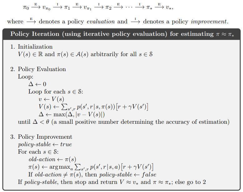
The main loop of the policy iteration code in IntroRL is shown below.
while made_changes or (max_delta>err_delta):

    max_delta = dp_policy_evaluation( policy, state_value, do_summ_print=False,
                                      max_iter=max_iter, err_delta=err_delta, gamma=gamma)

    made_changes = dp_policy_improvement( policy, state_value, gamma=gamma,
                                         do_summ_print=False, max_iter=max_iter)
Value Iteration
The approach to value iteration is defined in Sutton & Barto pages 82 to 84 as follows.
It includes alternating between truncated versions of policy evaluation and policy improvement. It avoids the need for those policy functions to reach their own, individual termination criteria.
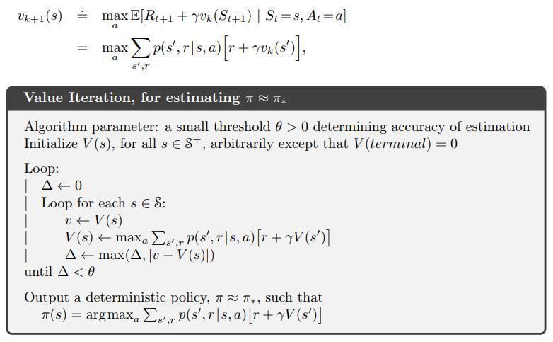
The main loop of the value iteration code in IntroRL is shown below.
while (loop_counter<max_iter) and (not all_done):
    loop_counter += 1
    all_done = True
    delta = 0.0 # used to calc largest change in state_value

    for s_hash in policy.iter_all_policy_states():
        VsD = {} # will hold: index=a_desc, value=V(s) for all transitions of a_desc from s_hash

        # MUST include currently zero prob actions
        for a_desc, a_prob in policy.iter_policy_ap_for_state( s_hash, incl_zero_prob=True):
            calcd_v = 0.0

            for sn_hash, t_prob, reward in \
                environment.iter_next_state_prob_reward(s_hash, a_desc, incl_zero_prob=False):

                calcd_v += t_prob * ( reward + gamma * state_value(sn_hash) )

            VsD[a_desc] = calcd_v

        best_a_desc, best_a_val = argmax_vmax_dict( VsD )
        delta = max( delta, abs(best_a_val - state_value(s_hash)) )
        state_value[s_hash] = best_a_val

    if delta > error_limit:
        all_done = False
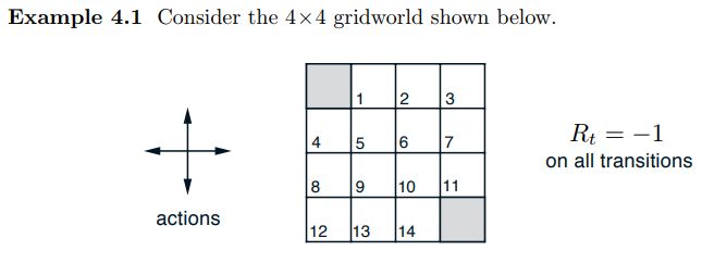
Example 4.1 Gridworld
The gridworld in Example 4.1 on pages 76 and 77 of Sutton & Barto is used to demonstrate the convergence of policy evaluation.
It is a small gridworld with 4 equiprobable actions and a -1 reward for every action.
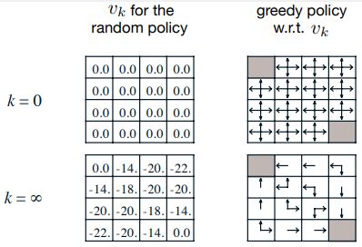
The image below is a portion of figure 4.1 that shows the value function and policy that result from applying policy evaluation repeatedly to convergence.
The code block below calls the IntroRL policy evaluation function to arrive at the same result.
from introrl.dp_funcs.dp_policy_eval import dp_policy_evaluation
from introrl.policy import Policy
from introrl.state_values import StateValues
from introrl.mdp_data.sutton_ex4_1_grid import get_gridworld

gridworld = get_gridworld()

pi = Policy( environment=gridworld )
pi.intialize_policy_to_equiprobable( env=gridworld )

sv = StateValues( gridworld )
sv.init_Vs_to_zero()

dp_policy_evaluation( pi, sv, max_iter=1000, err_delta=0.001, gamma=1., fmt_V='%.1f')
The output from the above code is:
Exited Policy Evaluation
   iterations     = 167  (limit=1000)
   measured delta = 9.620565251111657e-07
   gamma          = 1.0
   err_delta      = 0.001
   error limit    = 1.0010010010010018e-06
   STOP CRITERIA  = 0.0010010010010010019

___ "Sutton Ex4.1 Grid World" State-Value Summary ___
 === Sutton Ex4.1 Grid World ===
            0  1  2  3  ||
            4  5  6  7  ||
            8  9 10 11  ||
           12 13 14  0  ||
 ========== State-Hash =========
     ___ Sutton Ex4.1 Grid World State-Value Summary, V(s) ___
                        0.0 -14.0 -20.0 -22.0  ||
                      -14.0 -18.0 -20.0 -20.0  ||
                      -20.0 -20.0 -18.0 -14.0  ||
                      -22.0 -20.0 -14.0   0.0  ||
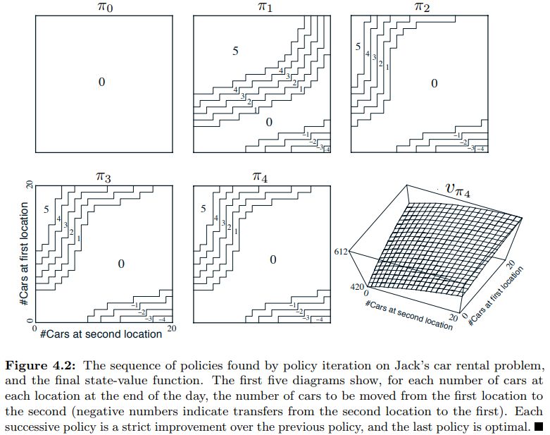
Figure 4.2 Car Rental
The Car Rental Problem on page 81 of Sutton & Barto is used to demonstrate the convergence of policy iteration.
For a description of the problem, see page 81 of Sutton & Barto , however, the results of the policy iteration are shown below.
The code block below calls the IntroRL policy iteration function to arrive at the same result.
from introrl.dp_funcs.dp_policy_iter import dp_policy_iteration
from introrl.policy import Policy
from introrl.state_values import StateValues
from introrl.mdp_data.car_rental import get_env
env = get_env()
policy = Policy( environment=env )
policy.intialize_policy_to_random( env=env )
state_value = StateValues( env )
state_value.init_Vs_to_zero()
dp_policy_iteration(policy, state_value,
do_summ_print=True, show_start_policy=True,
max_iter=1000, err_delta=0.0001, gamma=0.9)
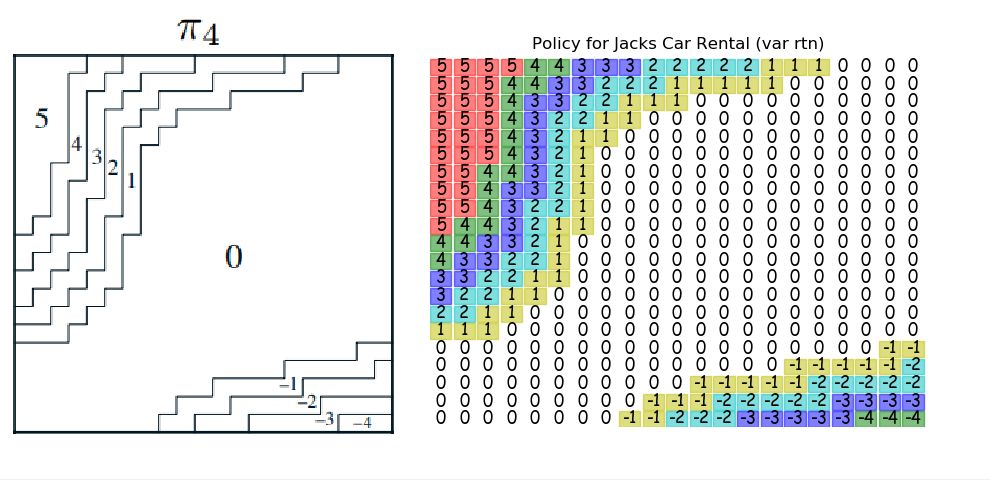
diag_colorD = {'5':'r', '4':'g', '3':'b', '2':'c', '1':'y', '0':'w',
'-5':'r', '-4':'g', '-3':'b', '-2':'c', '-1':'y'}
policy.save_diagram( env, inp_colorD=diag_colorD, save_name='car_rental_var_rtn')
The policy diagram from the output of the above code is compared to the textbook answer below.
The 3D plot of the state value from the output of the above code is compared to the textbook 3D plot.
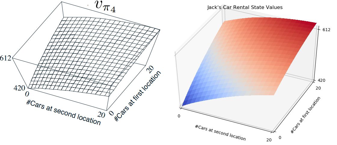
The 3D plot above is created by first running a script to make a data file, Car Rental, Make Data File Code
And then running a script to create Car Rental, 3D Plot Souce Code
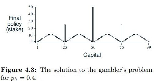
Figure 4.3 Gambler’s Problem
The Gambler’s Problem on page 84 of Sutton & Barto is used to demonstrate value iteration.
For a description of the problem, see page 84 of Sutton & Barto , however, the results of the policy iteration are shown below.
The code block below calls the IntroRL value iteration function to arrive at the same result.
The answer from IntroRL is the full answer (i.e. referred to in the problem description). Only the minimum bet policy is shown in the textbook answer.
Both plots are shown below.
from introrl.dp_funcs.dp_value_iter import dp_value_iteration
from introrl.mdp_data.gamblers_problem import get_gambler

gambler = get_gambler(prob_heads=0.4)

policy, state_value = dp_value_iteration( gambler, allow_multi_actions=True,
                                          do_summ_print=True,fmt_V='%.4f',
                                          max_iter=1000, err_delta=0.00001,
                                          gamma=1.0)
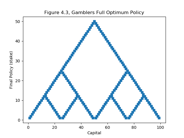
Both of the charts above are created with the Gambler’s Problem Run and Plot Souce Code